Top 6 Object Detection Algorithms

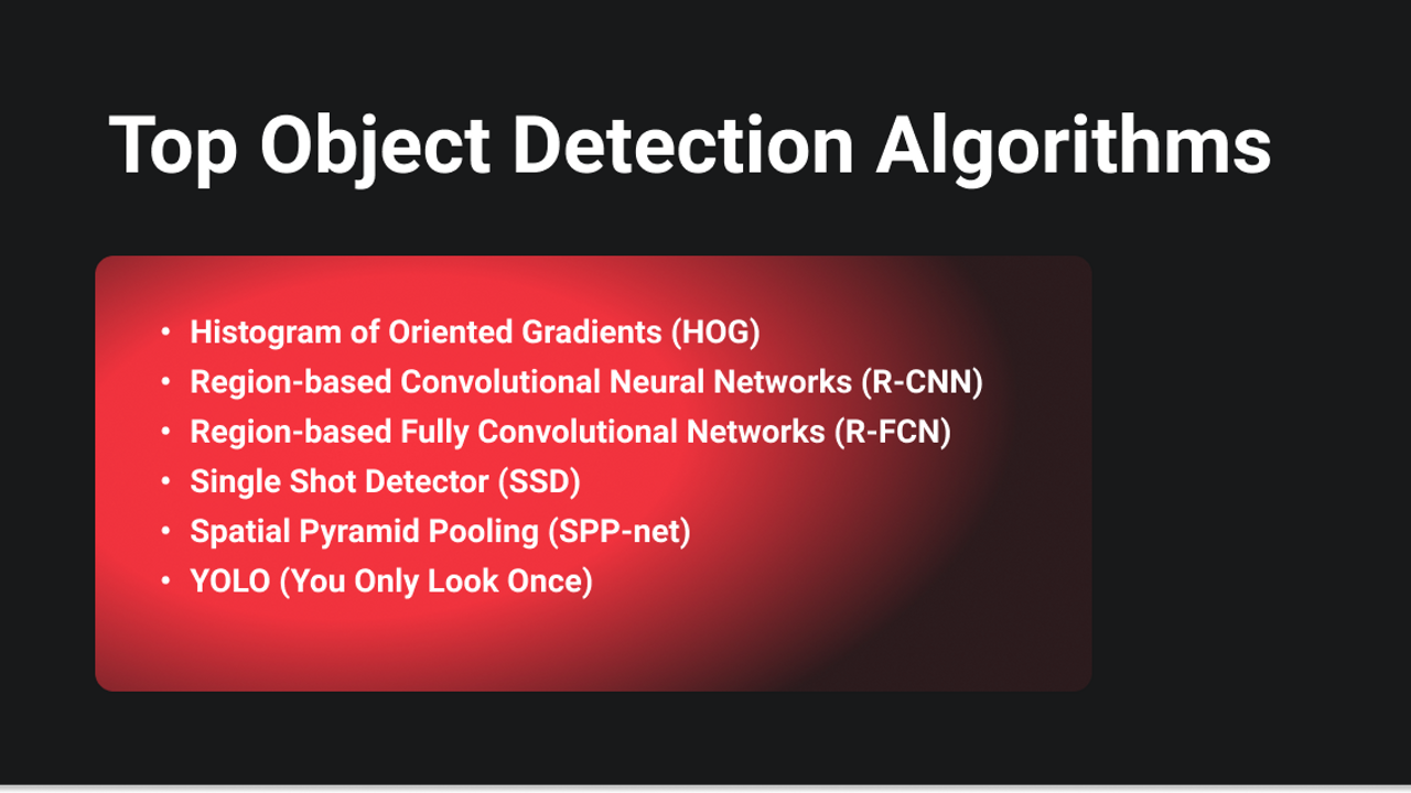
Object detection is a computer vision task that aims to identify and locate objects in an image or video. This identification and localization make object detection suitable for things like counting objects in a scene, determining and tracking their precise locations, all while labeling them. In this post, we will go through the six most prevalent object detection techniques.

Histogram of Oriented Gradients (HOG) Feature Descriptor

Feature descriptors take an image and compute feature descriptors/vectors. These features act as a sort of numerical “fingerprint” that can be used to differentiate one feature from another. The Histogram of Oriented Gradients(HOG) algorithm counts the occurrences of gradient orientation in localized portions of an image. It divides the image into small connected regions called cells, and for the pixels within each cell, the HOG algorithm calculates the image gradient along the x-axis and y-axis.

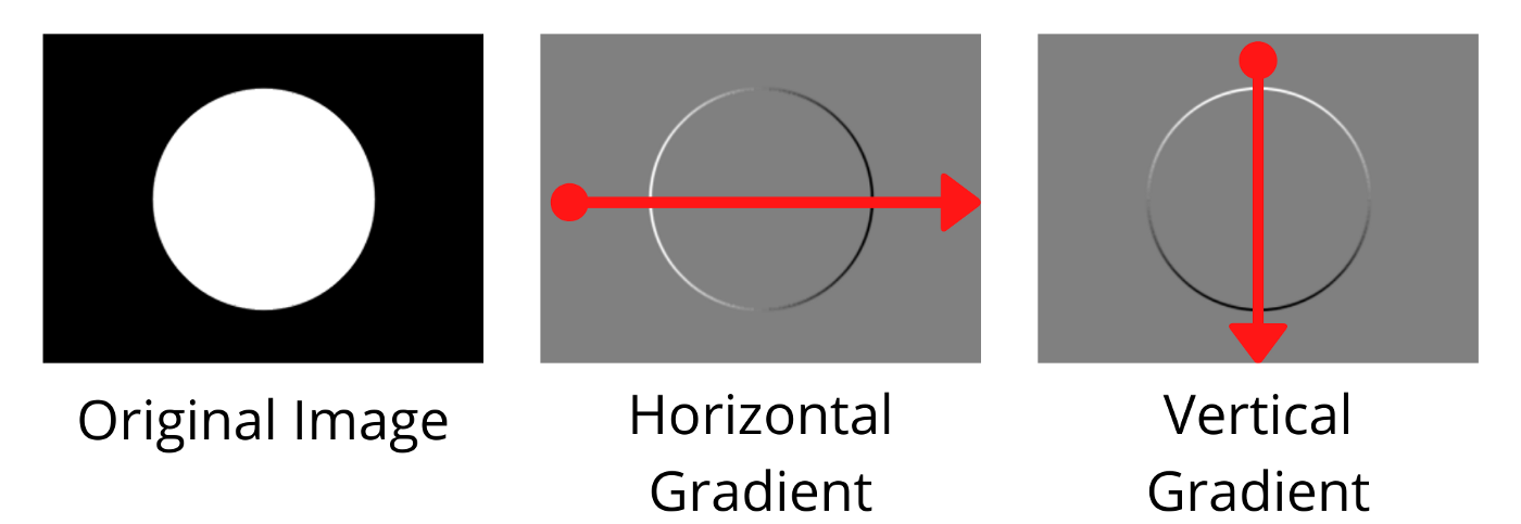
Pixel-wise gradients visualized

These gradient vectors are mapped from 0–255, pixels with negative changes are black, pixels with large positive changes are black, and pixels with no changes are grey. Using these two values, the final gradient is calculated by performing vector addition.

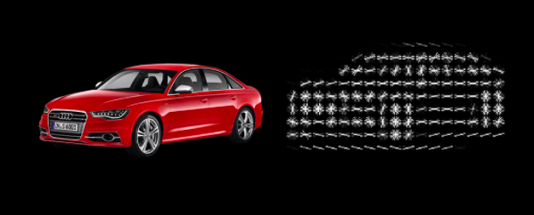
HOG features for a car

Let’s say we are using 8x8 pixel-sized cells, after obtaining the final gradient direction and magnitude for the 64 pixels, each cell is split into angular bins. Each bin corresponds to the gradient direction, with 9 bins of 20° for 0–180°. This enables the Histogram of Oriented Gradients (HOG) algorithm to reduce 64 vectors to just 9 values. HOG is generally used in conjunction with classification algorithms like Support Vector Machines(SVM) to perform object detection.

Region-based Convolutional Neural Networks (R-CNN)

R-CNN architecture

Convolution Neural Networks (CNNs) are not able to handle multiple instances of an object or multiple objects in an image. R-CNN first performs selective searchto extract many different-sized region proposals from the input image to work around this limitation. Each of these region proposals is labeled with a class and a ground-truth bounding box. A pre-trained CNN is used to extract features for the region proposals through forward propagation. Next, these features are used to predict the class and bounding box of this region proposal using SVMs and linear regression.

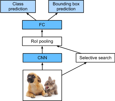
Fast R-CNN architecture

R-CNN selects thousands of region proposals and independently propagates each of these through a pre-trained CNN. This slows it down considerably and makes it harder to use for real-time applications. To overcome this bottleneck Fast R-CNN performs the CNN forward propagation once on the entire image.

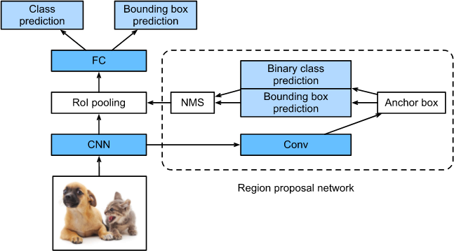
Faster R-CNN architecture

Both R-CNN and Fast R-CNN produces thousands of region proposal, most of which are redundant. Faster R-CNN reduces the total number of region proposals by using a region proposal network(RPN) instead of selective search to further improve the speed.

Region-based Fully Convolutional Network (R-FCN)

The R-CNN family of object detectors can be divided into two sub-networks by the Region-of-Interest (ROI) pooling layer:

1. A shared, “fully convolutional” subnetwork independent of ROIs
2. An ROI-wise subnetwork that does not share computation.

ROI pooling is followed by fully connected (FC) layers for classification and bounding box regression. The FC layers after ROI pooling do not share among different ROIs and take time. This makes R-CNN approaches slow, and the fully connected layers have a large number of parameters. In contrast to region-based object detection methods, Region-based Fully Convolutional Network (R-FCN) is fully convolutional with almost all computation shared on the entire image.

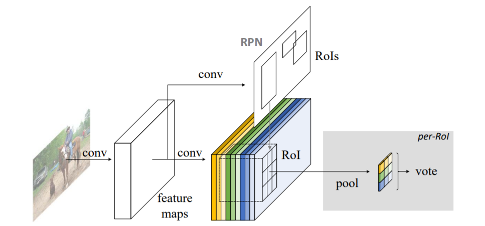
R-FCN architecture

R-FCN still uses an RPN to obtain region proposals, but in contrast to the R-CNN family, the fully connected layers after ROI pooling are removed. Rather, all major computation is done before ROI pooling to generate the score maps. After the ROI pooling, all the region proposals use the same set of score maps to perform average voting. So, there is no learnable layer after the nearly cost-free ROI layer. This reduces the number of parameters significantly, and as a result, R-FCN is faster than Faster R-CNN with competitive mAP.

Single Shot Detector (SSD)

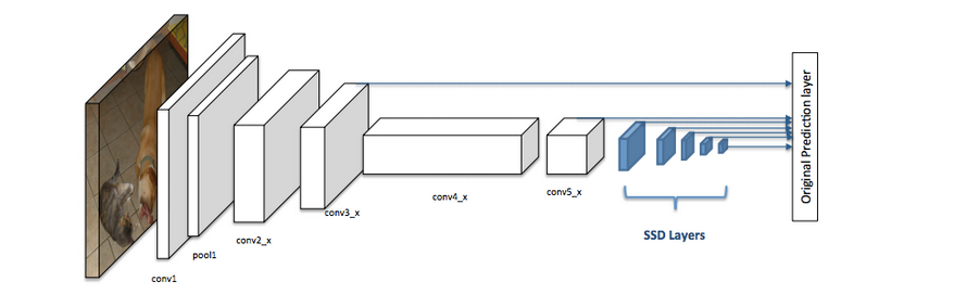
Single Shot Detector (SSD) architecture

Single Shot Detector (SSD) has two parts:

• a backbone model for extracting features
• an SSD convolutional head for detecting objects.

The backbone model is a pre-trained image classification network (like ResNet) from which the last fully connected classification layer has been removed. This leaves us with a deep neural network that can extract semantic meaning from the input image while preserving the spatial structure of the image. The SSD head is simply one or more convolutional layers added to this backbone model. The outputs are interpreted as the bounding boxes and classes of objects in the spatial location of the activations of the final layers.

Spatial Pyramid Pooling (SPP-net)

CNNs require a fixed-size input image, which limits both the aspect ratio and the scale of the input image. When used with arbitrary sized images CNNs fit the input image to the fixed size via cropping or warping. However, cropping might result in the loss of some parts of the object, while warping can lead to geometric distortion. Furthermore, a pre-defined scale does not work well with objects of varying scales.

CNNs consist of two parts: the convolutional layers, and fully connected layers. The convolutional layers work in a sliding window manner do not require a fixed image size and can generate feature maps of varying sizes. The fully connected layers, or any other classification algorithm like SVM for that matter, requires fixed-size input. Hence, the fixed-size constraint comes only from the fully connected layers.

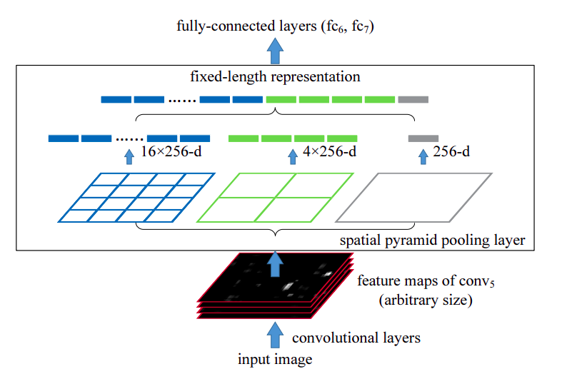
Network structure with a spatial pyramid pooling layer

Such input vectors can be produced by the Bag-of-Words (BoW) approach that pools the features together. Spatial Pyramid Pooling (SPP) improves upon BoW, it maintains spatial information by pooling in local spatial bins. These bins have sizes proportional to the image size, this means the number of bins remains unchanged regardless of the image size. To use any deep neural network with images of arbitrary sizes, we simply replace the last pooling layer with a spatial pyramid pooling layer. This not only allows arbitrary aspect ratios but also allows arbitrary scales.

SPP-net computes the feature maps from the entire image once and then pools the features in arbitrary regions to generate fixed-length representations for the detector. This avoids repeatedly computing the convolutional features. SPP-net is faster than the R-CNN methods while achieving better accuracy.

YOLO (You Only Look Once)

The YOLO — You Only Look Once — network uses features from the entire image to predict the bounding boxes, moreover, it predicts all bounding boxes across all classes for an image simultaneously. This means that YOLO reasons globally about the full image and all the objects in the image. The YOLO design enables end-to-end training and real-time speeds while maintaining high average precision.

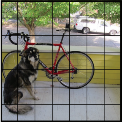
S x S grid

YOLO divides the input image into an S × S grid. If a grid cell contains the center of an object, it is responsible for detecting that object. Each grid cell predicts B bounding boxes and confidence scores associated with the boxes. The confidence scores indicate how confident the model is that the box contains an object, and additionally how accurate the box is. Formally, the confidence is defined as P(Objectness) x IOU_truthpred. Simply put, if no object exists in a cell, the confidence score becomes zero as P(Objectness) will be zero. Otherwise, the confidence score is equal to the intersection over union (IOU) between the predicted box and the ground truth.

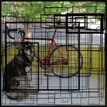
Bounding boxes and confidence scores

Each of these B bounding boxes consists of 5 predictions: x, y, w, h, and confidence. The (x, y) coordinates represent the center of the box relative to the bounds of the grid cell. The width(w) and height(h) are predicted relative to the whole image. The confidence prediction represents the IOU between the predicted box and any ground truth box.

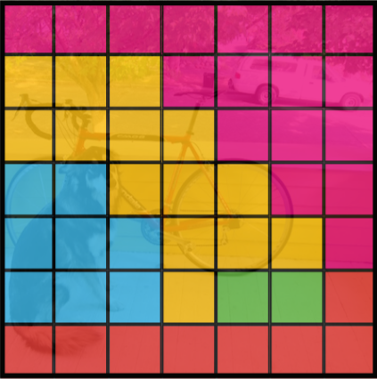
Class probability map

Each grid cell also predicts C conditional class probabilities, P(Class-i |Object). These probabilities are conditioned on the grid cell containing an object. Regardless of the number of associated bounding boxes, only one set of class probabilities per grid cell is predicted.

Final detections

Finally, the conditional class probabilities and the individual box confidence predictions are multiplied. This gives us the class-specific confidence scores for each box. These scores encode both the probability of that class appearing in the box and how well the predicted box fits the object.

YOLO performs classification and bounding box regression in one step, making it much faster than most CNN-based approaches. For instance, YOLO is more than 1000x faster than R-CNN and 100x faster than Fast R-CNN. Furthermore, its improved variants such as YOLOv3 achieved 57.9% mAP on the MS COCO dataset. This combination of speed and accuracy makes YOLO models ideal for complex object detection scenarios.

YOLOR, You Only Learn One Representation, is the best YOLO variant to date. YOLOR has a unified network that integrates implicit knowledge and explicit knowledge. It pre-trains an implicit knowledge network with all of the tasks present in the COCO dataset to learn a general representation, i.e., implicit knowledge. To optimize for specific tasks, YOLOR trains another set of parameters that represent explicit knowledge. Both implicit and explicit knowledge are used for inference.

This list is by no means exhaustive, there are a plethora of object detection techniques beyond the ones mentioned here. These are just the ones that have seen widespread recognition and adoption so far.

Object Detection and Tracking using YOLOR and DeepSort

Do you want to learn more about object detection algorithms and make amazing applications like the one shown above? Enroll in our YOLOR object detection course here! It is a comprehensive course that covers object detection fundamentals, implementation, and building various applications, as well as integrating models with a StreamLit UI for building your computer vision web apps.